TUTORIEL | Spark Structured Streaming: from data management to processing maintenance

Spark is an open source distributed computing framework that is more efficient than Hadoop, supports three main languages (Scala, Java and Python) and has rapidly carved out a significant niche in Big Data projects thanks to its ability to process high volumes of data in batch and streaming mode. Its 2.0 version introduced us to a new streaming approach known as Structured Streaming. What is it all about? Well, we invite you to read this series of 3 articles to find out. Let’s go!

How Spark Structured Streaming works

Structured Streaming allows you to process flowing data streams using the Spark SQL library and standard objects such as DataFrames or Datasets. This approach replaces the previous Spark Streaming library which had the huge downside of handling objects as DStreams.

By placing the SQL library at the heart of the project and using it for both batch and stream processing as well as machine learning, the team in charge of Spark thus continues to unify to unify the framework.

But let’s get back to streaming.

Stream processing can be seen as a 3-step process:

• Stream read (in our case, a Kafka topic)
• Data transformation
• Writing to target (in our case, two targets HDFS and PostgresSQL)

For the Kafka read, we can proceed as follows.

def readFromKafka(topic: String, bootstrapServers: String): Dataset[String] = {
  val df = spark.readStream
    .format("kafka")
    .option("kafka.bootstrap.servers", bootstrapServers)
    .option("subscribe", topic)
    .option("startingOffsets", "latest")
    .option("failOnDataLoss", value = false)
    .load()`
    .select(col("value))
  }

We then store the received data on HDFS. To do so, we simply write a basic function that takes our previously mentioned DataFrame as input. We also give it 3 additional settings:

• Path: the location in which to store the data
• CheckpointHdfsPath: the location in which to store checkpoint information (we will see why this is useful later)
• TriggerDelay:  the time delay, in ms, between two write operations (and yes, we are still operating in micro-batch mode) 

def writeToHdfs(df: DataFrame, path: String, checkpointHdfsPath: String, triggerDelay: Long = 60000L): StreamingQuery = {
    df.writeStream
      .trigger(Trigger.ProcessingTime(triggerDelay))
      .format("parquet")
      .option("path", path)
      .option("checkpointLocation", checkpointHdfsPath)
      .outputMode(OutputMode.Append())
      .start()
  }

Micro-batch means that Spark will generate code that will be executed at regular intervals. This frequency can be defined using the trigger option. If processing takes longer than the interval between 2 executions, it does not really matter: executions that should have been launched during that time period are just forgotten.If the processing takes too long, then data could start building up in Kafka, which means that more time will be needed to process it. The phenomenon should thus not be allowed to persist.

For the storage on Postgres, the same principle applies except that we indicate the name of a table rather than a path.

def writeToPostgre(data: DataFrame, table: String, triggerDelay: Long = 60000L): StreamingQuery = {
    agg.writeStream
      .trigger(Trigger.ProcessingTime(triggerDelay))
      .outputMode(OutputMode.Update())
      .foreach(writerSQL(table))
      .option("checkpointLocation", checkpointCkdbPath)
      .start()
  }

In our use case, we will first aggregate the data over a time frame before writing the result in Postgres. We will take a closer look at this later.

Spark generates independent queries for each streamed write

Stéphane Walter

Technically, writing to a database is a more complex operation, especially with the 2.3.0 version of Spark that we use. This is why we have chosen to use the `foreach(writerSQL(table))` instruction. I will not go into further details about this section in the present article as this would take us too far. Just know that we are inserting the data into the database in upsert mode.

The key thing to understand about Structured Streaming is that Spark generates independent queries for each stream writing. This is never mentioned in documentation which tends to focus on extremely simple cases.

So, how will this be reflected in our example?

• A first query that will read the Kafka data and then store it on HDFS.
• A second query that will read the Kafka data, aggregate it and then insert it into a Postgres table.

You could think that the Kafka read would only be executed once, with the half-stream then feeding two separate output streams in a Y-shaped configuration.

But, if you are planning to use the aggregated data to populate, not 1 but 5 tables for example, this will generate 5 separate processing instances and consequently 5 distinct Kafka reads, 5 aggregate computations and 5 writing operations to the base. This means that performance will naturally deteriorate.

In such a case, we recommend that you populate only 1 table with aggregate data of sufficient granularity and then build views in the base to recreate other requested tables. This option has the advantage of simplicity. No interdependence between queries. Each query is autonomous and manages its own interruptions, trims and problems through checkpoints.

It is now time to programme the queries. This can be done as follows.

val input = readFromKafka("topicTest", "kafka:9092")
val outputHdfs = writeToHdfs(input, "testHdfs", "ckpHdfs")
val data = normalize(input)
val agregat = aggData(data)
val outputDb   = writeToPostgres(agregat, "testTable", "ckpTable")
spark.streams.awaitAnyTermination(TIMEOUT)

This last instruction is crucial. It is the one that will command Spark to run the queries until the TIMEOUT value is reached. We will choose this timeout value later.

The complexities of streaming

Managing late data

• What happens when data is late?
• Should it be included in computations?
• If a piece of data arrives one day late, should I recompute yesterday’s aggregate?
• If a piece of data arrives one year late, should I recompute yesterday’s, last week’s, last month’s, etc., aggregate?

Spark offers a smart solution (only for aggregate computations): the watermark.

The watermark will set the acceptable limit for late data. Beyond, the data will not be taken into account. This will help Spark purge data stored in the memory.

But how does this work?

To understand, we need to take a closer look at the method used to compute aggregates.

def aggData(df: DataFrame, watermark: String = "60 seconds"):DataFrame = {
    df.select("requestId", "hostname", "status","datum", "bytes")
      .withWatermark("datum", watermark)
      .groupBy(window($"datum", "60 seconds","60 seconds"), $"hostname", $"status")
      .sum("bytes")
      .withColumnRenamed("sum(bytes)","bytes")
      .withColumn("datum",$"window.start")
  }

Now let’s detail our method.

We receive a DataFame as input and only keep 5 columns:

• requestId: a unique identifier for the record
• hostname: a machine name that will be used as dimension
• status: a status that will also be used as dimension
• datum: record time and date in timestamp format
• bytes: number of bytes transmitted by the machines

We are thus going to aggregate bytes over a 60s time frame, and this aggregate will also be computed every 60s. The watermark requires that input data have to be timestamped.

In our example, this role is fulfilled by the datum field.

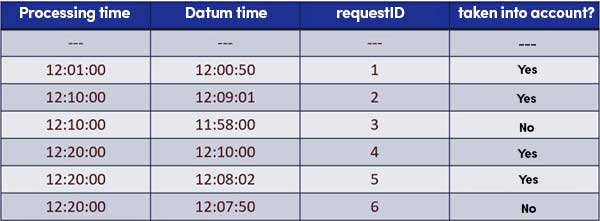
Some explanations regarding these results, a few of it may surprise those unfamiliar with Spark Structured Streaming.

1. Line 2 (Timestamp time 12:00:50) – It is the first record, so it is included.
2. Line 3 (Timestamp time 12:09:01) – The record is less than one minute late so it is included. What is this lateness that we are talking about?
3. Line 4 (Timestamp time 11:58:00) – The record is more than 60s late, so it is not included.
4. Line 5 (Timestamp time 12:10:00) – At first sight, the most surprising result: that piece of data arrives more than 10 min late and yet, Spark will keep it to compute its aggregate. This is simply because lateness is not determined with respect to processing time but rather with respect to data reception time. At the time when I am processing this data, the last piece of data was received at 12:09:01 so this record is not late.
5. Line 6 (Timestamp time 12:08:02) – Same reasoning. Note that record 4 is not included because it was processed in the same batch (the same micro-batch).
6. Line 7 (Timestamp time 12:07:50) – Here, on the other hand, the record is precisely 71s late with respect to record 2: consequently, it is not included.  µ

The Kafka read

Kafka does not manage much: it is the consumer that asks Kafka for the messages he wants to read. The technical term used is OFFSET and refers to a sort of data index.

For this project, we have set the offset to latest in the read parameters. Which means that when Spark starts, it begins to read only as from the latest message (forgetting about all the previous messages). This is essential when dealing with projects involving huge volumes of data.

• What happens when processing crashes or stops?
• Will it restart as from the latest message because of this latest setting? No

Spark will check the checkpoints file and restart as from the last processed offset.

Consequently, if the platform is unavailable for a really long time (but not Kafka), it is extremely important that you purge checkpoints. Otherwise, the operation will try to process the whole stock of accumulated messages and may never catch up on the backlog.

Kafka duplicates

Kafka guarantees message delivery but not its uniqueness. This means that Kafka can send the same message several times.

This is not a systematic problem.

There is a simple command in Spark to manage this: dropDuplicates.

def aggData(df: DataFrame, watermark: String = WATERMARK_VALUE):DataFrame = {
    df.select("requestId", "hostname", "status","datum", "bytes")
      .withWatermark("datum", watermark)
      .dropDuplicates("datum", "request_id")
      .groupBy(window($"datum", "60 seconds","60 seconds"), $"hostname", $"status")
      .sum("bytes")
      .withColumnRenamed("sum(bytes)","bytes")
      .withColumn("datum",$"window.start")
  }

Remember to call up the name of the column to which the watermark applies if you do not want to risk memory leaks with Spark keeping the whole history when executing its dropDuplicates.

Since detailed data is not deduplicated, this means that the distinct function must be used when performing analyses.

Stream processing maintenance

If you are working on a production cluster, you have certainly set up Kerberos to secure the connections between the machines. But Kerberos tickets have a limited lifespan. After some time (approximately 4 days), the ticket expires and the processing triggers an error due to a rights issue.

Generally, it is best to avoid killing processing in an abrupt manner whenever possible. How then to proceed to update a job or renew a Kerberos ticket?

We recommend setting up a scheduled interruption of processing during an off-peak period using a timeout in the awaitTermination instruction.

spark.streams.awaitAnyTermination(TIMEOUT)

In order to schedule a fixed time interruption (03:00), we have created a function that automatically computes the timeout value based on the actual launch time. Once stopped, it can simply be restarted with a scheduler as for batch processing.

And thanks to checkpoint, these periodic downtimes will not cause the loss of any messages. This is where this first article ends. In the next post, we will focus on data transformation, quality control and unit testing.